Useful formulas in the canonical ensemble

In the canonical ensemble we hold fixed the inverse-temperature . The goal is to compute the partition function . Suppose we find

We can compute the entropy

One special case is which we get in the case of an extremal black-hole. The entropy is a constant and gives us the extremal entropy.

The other special case is which is an important correction in the SYK model. The entropy is proportional to the temperature. This has been dubbed the “near-extremal” entropy.

Useful formulas in the microcanonical ensemble

In the microcanonical ensemble, we fix the energy and ask: What is the entropy as a function of ? Suppose we find a power law, that is,

The next step is to compute the temperature

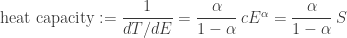
We also want to compute the heat capacity

We see that for the heat capacity to be positive, we must have . Indeed for a CFT in spacetime dimensions, obeys these bounds.

The Hagedorn case corresponds to and we see that the temperature is independent of the energy, and the heat capacity is infinite. This is like a mixture of water and ice at the freezing point. We also have the equality since .

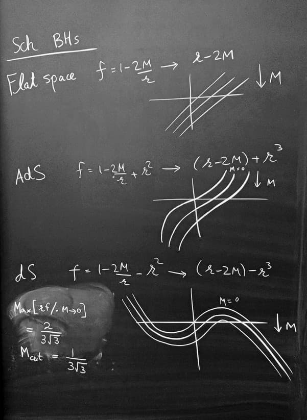
The Schwarzschild black hole in four dimensions, we have and we have a negative heat capacity, famously so.

Harmonic oscillator partition function using path integrals

Two pages of notes explaining how to derive the partition function of the harmonic oscillator using the path integral. Care is needed in normalizing the measure, and relatedly, to deal with the Matsubara zero mode of the free particle.

Harmonic oscillator path integral

Schwarzschild free energy

Two pages of notes on computing the Schwarzschild free energy in 4 dimensions, following the 1977 paper of Gibbons and Hawking.

Schwarzschild Free Energy

Videos of some talks I’ve given

2015 Kavli Institute, Santa Barbara, California

http://online.kitp.ucsb.edu/online/entangled15/mahajan/

 

2016 Perimeter Institute, Waterloo, Canada

http://perimeterinstitute.ca/videos/transport-chern-simons-matter-theories

 

2018 Kavli Institute, Santa Barbara, California

http://online.kitp.ucsb.edu/online/chord18/mahajan/

 

Degree of the identity map on S^2

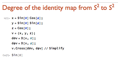
The winding number of the identity map from to  should be one, and we can check this using the following Mathematica code.

Denoting the triple product of 3-vectors by square brackets, the general expression is

.

Comparing Sch. black holes with different CC

We will restrict to 3+1 dimensions, and compare the emblackening factors.

Internal spin of a dyon

The normalization of gauge fields means that the magnetic charge of the fundamental magnetic monopole is . (It’s magnetic field is , so the flux through the sphere is .)

Dirac quantization then tells us that the electric charge is an integer.

Now let us look at the time derivative of the angular momentum of an electric charge moving in the field of a magnetic monopole with field .

.

Thus, even though angular momentum is not conserved, we can define a new quantity , which is conserved.

Now if the electric charge and the monopole were to form a bound state, the above calculation strongly suggests that we assign an internal spin to the dyon of magnitude . For the fundamental values and , we get spin .

Fibonacci and Ising anyons

(This post is very naive, and is only intended to serve as an aid to memory of various facts.)

Fibonacci

There are two types of anyons: 1 and . The nontrivial fusion rule is

.

This is as if we projected down to the -even sector of the 3D Ising model, and is thought of as the operator.

These anyons are related to the Read-Rezayi state and are thought to have something to do with the quantum hall state. Fibonacci anyons are non-abelian and provide a gate set which is universal for quantum computation.

Ising

There are three types of anyons: 1, and . The fusion rules are the same as the OPE fusion rules of the 2D Ising model. (In the 2D Ising model, we have  instead of the more generic that we might expect from the symmetry. In the 3D Ising model, it is the second relation which is true.)

The correct Chern-Simons description of Ising anyons is the WZW model . This is also relevant for the Moore-Read state.

This system does have “non-abelian” anyons, but the gate set that one gets is not universal for quantum computation.

Green’s function method with boundary values

Let’s keep it simple. Suppose you want to solve the Laplace equation on a domain . The domain has boundary . You are given the source function in the domain , and the boundary condition .

The crucial point to note is that no matter what the specified boundary value , the Green’s function is defined to vanish on the boundary.

We start with the identity

Upon noting that satisfies the Laplace equation with a delta function source and that vanishes on the boundary, we get the solution for as

The first term encodes the bulk source, and the second term encodes the boundary value. Note that this shows up in AdS/CFT, where the “bulk-to-boundary” propagator is the radial derivative of the bulk-to-bulk propagator.